A scientific calculator contains functions that are used routinely by scientists and engineers. A good scientific calculator must be very precise and it must handle the huge dynamic range of numbers that are encountered in our understanding of science. Scientific calculators must often be used to extend our ability to make judgements based upon observations. This means that they must provide functions that help us analyze data as well as functions that simply calculate numbers.
A four function calculator can perform addition, subtraction, multiplication and division. These four basic functions represent the heart of any calculator. A Scientific calculator uses these four functions to perform higher level functions. For the purposes of this work, I arbitrarily segment the operations of a scientific calculator into the following categories:
Scientific electronic calculators are accurate. The precision of a calculator should be measured, rather than taking it for granted. Problems in accuracy can arise when repeated calculations are made on a single result. The nature of computational environment will determine the ultimate accuracy of long calculation. Precision is very important when doing division. Let's take a look at a quick example.
by definition, this value should equal 1. We have divided 1 by 3, 6 times and then multiply it by 3, six times. The problem with division by three stems from the fact that it is a repeating fraction that can never be represented with absolute accuracy. Multiple operations begin to accumulate errors.
The example cited above could also be expressed as
Each of these four expressions should yield exactly the same value (1 ). The mechanisms used by the calculator to determine each result is different.
The first expression just uses basic division and multiplication to perform the calculation. The second expression uses division, exponentiation , and multiplication. The third expression utilizes negative signed exponentiation, the final expression uses the logarithm to find a solution. If we carry out the calculations on a modern scientific calculator such as the HP32s and an older HP-97 we get the following table of errors:
|
|
HP-32sII | HP-97 |
| 1 | -1 X 10^-12 | -1 X 10^-10 |
| 2 | -9 X 10 ^-12 | -4 X 10^ -10 |
| 3 | -2 X 10^-12 | 0 |
| 4 | 0 | 0 |
From this short analysis, we see that the newer HP32sII has 2 more digits of accuracy than the HP-97.The newer calculator is 100X more precise than the older machine. Note that in the third equation, it appears that the older machine is more accurate. This could be the result of truncation in the exponent. The number of digits of in a calculation are often less consequential then the method used to round a number prior to calculation. These errors begin to manifest themselves in division calculations.
The wide dynamic range of the numbers used in scientific calculations leads to a requirement to represent numbers in terms of a mantissa and an exponent. The display of numbers on a calculator also requires some care in formatting. The formatting of a number was a particular challenge to designers of early calculators. The native language of the user often dictated the use of a comma where a decimal point might be used. This is difference is found in the differences in notation between English and German. The english value 1,234,567.89 is represented as 1.234.567,89. The differences in separators and other notation led to some difficulties in design of the machines. Users of HP calculators had a the ability to "fix" the display decimal point and select the presentation method to the display. Typical notations were SCI for scientific notation, ENG for engineering notation and FIX for fixed decimal point . Scientific notation uses a format of x.xxx X10^yy . Fixed point notation rounds the display to the required number of decimal points. Engineering Notation always presented an exponent that was divisible by 3.
There are two basic logical methods that can be used to describe the operation and entry of numbers on a calculator: Algebraic and Reverse Polish Notation (RPN). Each method has it's advantages and disadvantages. Many engineers perfer RPN machines because of their inherent clarity of operation. Others prefer Algebraic entry because of the similarity to hand calculation. Each method will be detailed a little later. First we'll explain a bit about the internal construction of a calculator. The calculator can be thought of like a house: there is an outside with it's facade and there is an inside which is unique to the design of the calculator. The keyboard of a caculator is like a door and the display of a calculator is like a window. While calculators differ in details, they all need a keyboard and a display. Entering a number into a calculator is just like entering a house through a door. Once you are inside, there are numerous directions you can go. When a number is pressed on the keyboard, it is displayed on a display to indicate that a choice has been made and the nature of that choice. The entry of numbers on calculator keyboard is based upon the Arabic Notion of reading a number from left to write.
Keyboard entry is the most basic algorithm found in a calculator. As each succeeding number is entered, the value in the keyboard register is multipled by 10 and the new number added to the result. When the decimal point is pressed, the value that is entered is divided by 10 to the power of the decimal point and added to the result. Each press of a key must be examined for validity and pupose. The left to right entry of the number system is natural for the human but someone complex at the machine level.
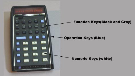
The keyboard can be divided into three distinct functional groups: Numeric, Operation, and Function. This distinct division can be seen on many early calculators. The HP-35 is a good example
As a general rule, function keys affect the value in the display, operation keys manipulate memory, and numeric keys enter numbers into the display.
Calculators utilize the concept of a register. A register is a place to store a number that will be affected by an immediate operation. Calculators also use standard memory registers that are used to to "hold" data or programs that will be used later in the process. The separation between an RPN logic calculator and an Algebraic machine is defined by a subtle difference between actions of the operation keys.
The Algebraic machine uses the operation key to move the number from the display register to an operand register. At the same time, the implied function of the operation key is "tagged" to this register. A new number is then entered in the display register. If the "=" key or another numeric operation key is pressed, the calculation is performed and the result is displayed. If another operation key such as a "+" has been pressed the result is placed back in the operation register. Entry of another number and a depression of the "=" key will process the result and display it.
The RPN machine utilizes the concept of a "stack" of registers. These machines utilize a single key to "push" a value up the stack. An operation key such as a "+" causes the first value to be "popped" and added to the displayed value. Early calculators, like the HP35 had a four level stack, labled x,y,z,t . Data could be pushed up the stack and used later on in the calculation. For example the following example may be used:
Solve X = 1 + cos (3.8 * Pi)
1 <enter> 3.8 <enter> PI, X, cos, +
An algebraic machine would need the following key strokes
1 + ( 3.8 X PI) cos =
The number of keystrokes is the same , but the ordering of operations is different. Debate rages about which system is better for everyday use. Algebraic notation gets very messy when dealing with functions of two variables. For instance and operation such as Rectangular to polar conversion. Entering the data is not really a problem, the function key is treated as an operation key. That is to say we enter the x value, press->P enter the y value and then press "=". The problem is with the second value. How do we get that. The answer is different on each machine. RPN machines always have a stack and the ability to swap the x and y registers. This allows convient storage and display of data. Some early Algebraic machines actually used memory registers to store the answers to multivariable functions.
Sexagisimal numbers are useful in time and angle calculations. The unique nature of these numbers is that they are associated with measures that have audifferent modulos based upon the position in the numeric representation. For instance, a common representation for time might appear as 11:33:14.5 . The leading digits are hours and may be expressed modulo 12 or 24. The next set of numbers is minutes and this modulo 60 and carries over into the hours. The next set of digits is seconds which is also modulo 60, but it has a modulo ten fractional part. The easiest way to handle calculations involving time is to "cast" the time into absolute seconds from a given date. This avoids all modulo problems during the mathematical operations. At the end of the calculation, the time is recast back to the HH:MM:SS.XX format.
The Scientific calculator must work with numbers that extend over a wide numeric range with high precsion. In addition to this, a numeric entry is often subjected to a number of transformations before arriving at an answer. Early calculators had very limited space for programs so it was necessary to arrive at a balance of accurate algorithms that occupied minimum space. In many instances the result of one key press was maintained for use in the next function. This was clearly seen in the early Monroe calculators. The "2nd function" key truly acted on the result from the first press of the key AND it was pressed after the function key. This is in contrast to a modern calculator where the 2nd function key alters the meaning of the operation key. The older Monroe or Compucorp machines would calculate a SINE. Depressing the second function key would then calculate the COSINE. A modern machine would generally calculate the ARC SINE function. which is a completely different algorithm. As memory and calculation power increased, the need for cleaverness and ingenuity in algorithm development for basic calculation decreased.
The basis of any good scientific calculator starts with an excellent multiply and add capability. Without these two functions, no other functions can be derived. At face value, it would seem that this should be trivial, but it is important that most early calculators (as well as many modern machines) worked in base ten, BCD (Binary Coded Decimal) arithmetic. This eliminates some of the simpler binary shifting techniques to perform multiplication. The challenge to the earlier designer of calculator algorithms was to utitlize those multiply and additions to drive the solution to the rest of the functions.
The Elementary functions
For the purposes of this work, we'll define the elementary functions as :
with the possible exception of the hyperbolic functions, the early scientific calculator could be expected to include all those functions. While the need for these functions was well defined, the method of calculation given minimal memory and minimal cycle times was not so clear. Let's look at some methods and considerations:
Consider the need to calculate the SINE of an arbitray angle. The function is completely defined over the range of 4pi and it repeats over that interval for an infinite period. If we have the ability to limit all entries to a range of 0 to 4Pi, then we need only concentrate on the numeric solution within this range. This process is called "RANGE REDUCTION" and it is a fundamental element of all scientific calculators and is often responsible for large errors . In some cases the errors are real but quite small. Try taking the sin(x) where x = 10^22. This number is interesting because it can be exactly represented in IEEE-754 double precision format. The exact result is:
-0.8522008497671888017727.....
My HP49G calculator reports
-0.852200849762
The difference is in 5 parts in the 12 decimal place. Hardly something to worry about, but it does illustrate a practical limitiation in modern calculator technology. Of course, having a computer isn't necessarily a benefit. If we choose to calculate this value using single precision (IEEE-754) mathematics, the resultant answer would be:
-0.73408......
This relatively huge error(9 parts in the second decimal place) comes from the lack of precision in the input numeric representation.
The polynomial is the basic algorithm used in most early scientific calculators. Accurate polynomial descriptions to a function over a rather large interval can require polynomials of high degrees. For instance, approximating the function ln(1+x) over the range [-1/2,1/2] with an error less than 10E-8 will require a polynomial of degree 12. Note that this requires a transformation or range reduction first.
The use of tables and interpolation can produce excellent results but the memory requirements generally limited the use of tables in most calulators. The advantages of tables include speed and accuracy, but this is of no use if there wasn't enough memory.
The CORDIC algorithm was the basis of the handheld revolution. The key feature of the CORDIC algorithm is that it can be utilized in the calculation of all the elementary functions.